Here I want to provide a very brief introduction to instabilities in some generic spatial equations, and in particular reaction-diffusion systems on continuous and discrete (network) domains. Turing instabilities in such systems provide a way to generate spatially heterogeneous states of such systems which exhibit a variety of interesting and complex structures. Such patterns are often used to try and explain emergent structures in developmental biology, such as the stripes and spots on animal coat patterns.
I will begin with a theoretical approach to the simplest method for the most general problem, and then show how this applies to particular relevant examples. Throughout the following discussion there will be subtle technical points (particularly regarding analytic details such as regularity of functions, topology of sets, etc) but I will omit almost all nonessential technical points to try and just illustrate the ideas in a useful way.
1. Linear Instability Theory in 
Consider an autonomous system of ordinary differential equations given by,

where  for each
  and
and  is a sufficiently `nice’ map to guarantee, e.g., global in time existence of solutions. Let
  be an equilibrium, so that
  . If we perturb this equilibrium by a small amount, we can track how perturbations grow (or decay) by setting
  where
where  , and substituting this into the ODE above. We get an equation for
  which we can Taylor expand as,

where  is the Jacobian of the function evaluated at the equilibrium
  .
.
After canceling an  above, and neglecting the higher-order terms, we have that satisfies a simple linear system of equations involving the Jacobian of the original nonlinear function at the equilibrium state. From the theory of such linear systems, we know that its long-time behaviour is determined by the eigenvalues of , say
  . In particular, if we have that all of their real parts are negative, i.e.
  for all
  , then the equilibrium is stable to small perturbations. If instead
  for at least one eigenvalue, then perturbations will grow, and the original equilibrium is unstable. At the boundary states of marginal stability (
 for one or more eigenvalues, with
  for all others), the behaviour of perturbations is harder to classify. Away from these states, it turns out that the linear system above directly tells how trajectories of the original system evolve near the equilibrium, via the Hartman-Grobman Theorem.
So to find if an equilibrium point is linearly unstable, we can simply look for parameters or equilibria that admit eigenvalues with positive real part. Many aspects of different kinds of instabilities are studied in bifurcation theory (particularly local bifurcation theory, which studies instabilities of equilibrium points), but for now we will move on to instabilities in PDEs.
2. General Stability Theory
Here we will consider something analogous to the above linear instability theory for somewhat generic transport-type equations. Instability theory for PDEs can be much more involved, and involve complicated spectral questions which I will not address here, but instead refer you to these introductory notes. In what follows, I will essentially assume that all operators have only point spectra, or that we can otherwise ignore these technicalities.
Consider a vector-valued function  , with the spatial domain
  which will be taken as either a set of points in the case of discrete operators, or as a manifold sufficiently smooth to do calculus on (you can think of the interval,
 ![{\Omega=[0,L]}](https://s0.wp.com/latex.php?latex=%7B%5COmega%3D%5B0%2CL%5D%7D&bg=ffffff&fg=000000&s=0&c=20201002) , for some length
, for some length  , as the simplest example). Here we will also assume this manifold is compact (i.e. bounded and containing its boundary), though other possibilities exist. We then assume that these functions evolve according to the following reaction-transport system,
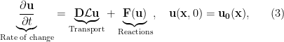
where  is a transport coefficient matrix,
  is a linear spatial operator, is a nonlinear function of
  , and
, and  is an initial spatial distribution. We remark that should be understood to contain whatever boundary conditions one might have, and can in general depend on the spatial variable
  , as well as derivatives with respect to this variable (but not in any way on time
  , as the non-autonomous setting is radically different).
A typical example which we will consider below would be the Laplacian on an interval, so that  where
where ![{x \in [0, L]}](https://s0.wp.com/latex.php?latex=%7Bx+%5Cin+%5B0%2C+L%5D%7D&bg=ffffff&fg=000000&s=0&c=20201002) . In this case we would also need to augment this operator with boundary conditions, e.g. the Neumann boundary conditions
. In this case we would also need to augment this operator with boundary conditions, e.g. the Neumann boundary conditions  . Here we will think of this operator as really a scalar operator acting linearly on each component of the function ; when this is not the case, and in particular when the spatial components of the system differ between equations, then one typically has trouble constructing eigenfunctions which are necessary to perform any kind of stability analysis, except in special cases. Finally we will also mention that in addition to restrictions of , one typically needs to consider elliptic operators and positive-definite matrices
  in order to ensure solutions to this system exist as time evolves. Blow-up of solutions and regularity are common mathematical questions that are studied for these kinds of systems. We make one further restriction on that it must annihilate constant vectors, so that a spatially homogeneous solution is determined purely by the function .
Next we will discuss stability of an equilibrium to this evolution equation against small spatial perturbations. As in the case of linear stability analysis for ordinary differential equations, perturbing an equilibrium solution will lead to a linear system, and for this reason we consider fundamental solutions to the linear operator . In the case of a compact domain and a suitable operator, these will be the set of eigenfunctions satisfying

Again we recall that for the Laplacian on an interval of length with Neumann conditions, we have that 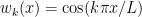 and
and  , with
  . In more complicated settings, such as being the Laplace-Beltrami operator on the sphere, or even the Laplacian on a planar square domain, there will be degeneracies such that many eigenfunctions correspond to given eigenvalues. Such degeneracies mean that analysis involving only the eigenvalues will not distinguish different eigenfunctions with the same eigenvalue. We can then assume that a solution to a linear equation involving can be expanded in a series of these functions as is typically done for separable linear partial differential equations.
With these assumptions in mind, we can then consider an equilibrium  to the evolution equation (3) which is spatially homogeneous so that
  . We assume the following ansatz for a perturbation to this equilibrium,

where  . Substituting (5) into (3) and using Taylor’s Theorem we find,

where is again the Jacobian of the nonlinear function evaluated at the steady state. We see that the the leading terms are satisfied by the equilibrium solution, so that up to corrections of order  , the perturbation satisfies a linear equation.
Hence using the arguments regarding separability as before, we can expand our perturbation in the form  and
and  is an undetermined constant vector. By linearity, while we can consider a general perturbation (which is a sum of infinitely many of the eigenfunctions indexed by
  ), they will evolve separately from one another and so studying them in isolation at this point is sufficient. We also note that the exponential here arises naturally in the setting of linear first-order systems, and hence
  fundamentally determines the long-time behaviour of the perturbation.
Substituting this particular form of the ansatz into (6), and considering only terms of  , we find the linear algebraic system,

where  is the identity matrix. In order for this linear system to admit nontrivial solutions, we require that the dimension of the nullspace of this matrix is nonzero. From linear algebra, this says that we must have
  , which provides an
  th degree polynomial relationship between and the eigenvalue
  . One can then look for things like conditions such that
  as varies to find that specific modes will grow in time, and it is these that lead to instabilities which can become spatially structured states (as long as the modes which grow are spatially structured; one typically assumes that the eigenvalues of are all negative, and hence in the absence of the spatial operator, the homogeneous equilibrium is stable).
3. Linear Analysis of Reaction-Diffusion Systems: Turing instabilities
We now apply the results to the case of instabilities of the homogeneous equilibrium of a two-component reaction-diffusion system on the interval ![{\Omega = [0,L]}](https://s0.wp.com/latex.php?latex=%7B%5COmega+%3D+%5B0%2CL%5D%7D&bg=ffffff&fg=000000&s=0&c=20201002) with Neumann boundary conditions. Writing
with Neumann boundary conditions. Writing  , we consider the system,
where the transport operator is now pure diffusion. We have the following quantities,

where the subscripts of  and
and  denote partial derivatives, and we assume the diffusion coefficients are both positive. Again the eigenfunctions and eigenvalues are given by
  and . We can then immediately apply the determinant condition above to find a quadratic equation determining for each eigenfunction , given by

While this expression seems complicated, it is easy enough to deduce requirements for a spatial instability. In particular, we note if the linear and constant term in this equation are both positive for some , this is equivalent to there being no values where and hence the homogeneous equilibrium is stable to perturbations of these modes. Similarly setting  (or equivalently, considering the system without diffusion) we can see that for a stable equilibrium in the homogeneous case, we require
  and
and 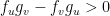 , which are the standard conditions for stability of a negative trace and positive determinant of the Jacobian of a planar system. Hence we then see that for any
  , the second term can never become negative, and so instability is possible only when the last term becomes negative, Assuming a continuum of eigenvalues , which is accurate for a sufficiently large domain, one can find algebraic conditions just in terms of model parameters, but here we will leave the eigenvalue in the condition, as it typically corresponds to the geometry. Murray’s Mathematical Biology gives a far more detailed treatment of these conditions and much more.
More generally, one can replace the Laplacian above by the Laplace-Beltrami operator on a manifold, and show that the growth rates are exactly determined by the above expression. The major difference is that the eigenvalues and eigenfunctions can be much more difficult to compute, and depend on the geometry in interesting ways. For examples of this, as well as simulations of pattern-forming instabilities with other operators, see the videos I have made for growing manifolds and reaction-advection-diffusion equations.
4. Instabilities in Network Reaction-Diffusion Systems
Given an undirected weighted graph (that is, with nodes or vertices and  edges
edges  ), we can use the adjacency matrix
  to describe a diffusion process between these nodes. In fact, this will involve something called the graph laplacian, which we will denote by
  . We think of having
  species at each node
  reacting with one another given by
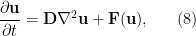
  , and diffusing to neighboring nodes. An analogue of the above reaction-diffusion system, given by (8), on a graph then looks like,

As this is a system of  equations, one could construct a Jacobian from the linearization about an equilibrium of the kinetics and simply compute the eigenvalues. Alternatively, as before, we can exploit the spectral properties of the matrix to find that perturbations to a homogeneous equilibrium will again have growth rates which satisfy Equation (10). The derivation of this fact replaces the eigenfunctions of
  above with the eigenvectors of , but is essentially unchanged.

